How to Use SUMIF in Google Sheets

Key takeaways

You can use the SUMIF function in Google Sheets to add numbers across a range of cells if they meet the conditions or to summarize data in a category.

• The use the SUMIF function, you use a syntax that defines the range of cells, the condition the function must meet, and, optionally, the range you want Google Sheets to use to add the numbers. 

• Like SUMIF, the SUMIFS function also adds a range of values based on the criteria you define. However, you would use SUMIFS for a range with multiple criteria and SUMIF to evaluate the data based on one criterion. 

• You can also perform various other Google Sheets functions to do even more with spreadsheets.

Learn how to sum up data that fits your stated criteria, such as a name, category, or dollar value, within a data set. Afterward, consider signing up for the Google Data Analytics Professional Certificate to continue building in-demand data analysis skills. Become familiar with critical tools and build your knowledge. Upon completion, you’ll earn a credential you can use to boost your resume and professional profile. 

The SUMIF formula in Google Sheets

The syntax for SUMIF is:

=SUMIF(range, criterion, [sum_range])

Within this formula, you’ll have the following components:

• Range: The range of cells to be evaluated by the criterion.

• Criterion: The condition to be met.

• Sum_range: (Optional) The range used to add up numbers. If this is omitted, then the first range is summed.

How to use SUMIF in Google Sheets

Ready to deepen your knowledge of Google Sheets?

To begin, you'll need your tab open to your spreadsheet. If you’re not already working with your own data set and want to follow along with our examples, make a copy of this template to practice. 

Once you have decided what information you’d like to sum up in this data set, click on any blank cell in the sheet to input the SUMIF formula. 

1. Select the range of cells to be summed up.

Use your mouse to drag and highlight (or type out) the alphanumeric range of cells that you’d like to sum up based on your criterion.

In our example, let’s say you want to know the total earnings of films directed by Steven Spielberg. Our range would be the column where Sheets will find “Steven Spielberg.”

Your inputs would look like:

• Range: The list of items that your criterion will be based on. In our practice sheet, that range would be C2:C47, or the list of directors.

• Criterion: The cell or criteria you are evaluating. In this case, you’ll type in “Steven Spielberg” (with the quotation marks).

• Sum range: The range of cells to be summed up. In the example, that would be F2:F47, the entire list of box office earnings.

Each of the above inputs is separated by commas and sits between two parentheses.

Read more: How to Use Data Validation in Google Sheets

2. Add the criterion.

Next, you’ll add the criterion to your formula. This can either be a number, text, or another cell. There are multiple options for SUMIF criteria, which are listed below. 

Using the practice example, add a comma and then "Steven Spielberg" to your formula.

3. Highlight the range of cells to be added up based on the criterion.

Drag (or type out) the alphanumeric range you’d like to sum up using your chosen criteria. This second range should be the range of cells containing amounts to be summed up. 

This step is optional and only necessary if your sum depends on data in a non-sum column.

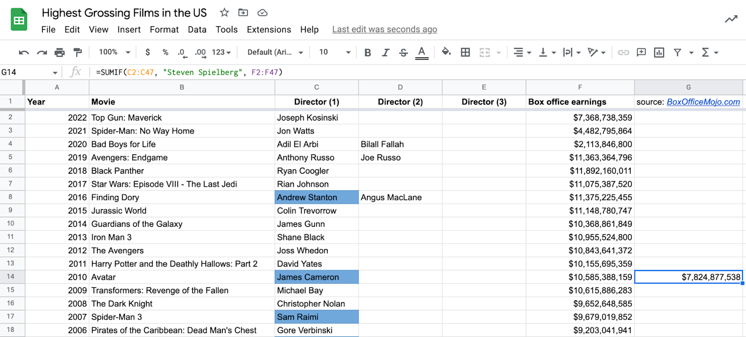
In the practice example, add a second comma. Then highlight the numbers (box office earnings) in column F to add F2:F47. At this point, your formula should look like this: 

=SUMIF(C2:C47, "Steven Spielberg", F2:F47)

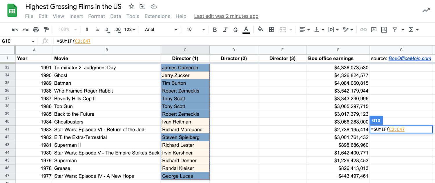
4. Press enter to sum up.

Close the parentheses to indicate a complete formula and press enter. Your sum will appear in the cell.

SUMIF vs. SUMIFS: What’s the difference?

Both SUMIF and SUMIFS functions add up a range of values based on criteria. The main difference is that SUMIF evaluates based on one condition at a time, while SUMIFS can check for multiple criteria. In the SUMIF formula, sum_range is the final (and optional) argument, but when using SUMIFS, sum_range is the first (and required) argument for SUMIFS.

SUMIF troubleshooting

Errors to look out for when using the SUMIF function:

• The #VALUE! error can occur if the SUMIF function refers to a cell or range in a closed workbook.

• The SUMIF formula can return incorrect values if you try to match strings that are longer than 255 characters.

• You may only use equal-sized ranges and sum_range in your formula. For example, if your range is C2:C47, your sum_range should reflect F2:F47 rather than F2:F100.

SUMIF limitations

When using the SUMIF function, these are some limitations and solutions to keep in mind.

• SUMIF cannot differentiate between uppercase and lowercase characters. If you have “steven spielberg” on your spreadsheet, SUMIF will still pick it up.

• SUMIF can return the sum of values “not equal to” the #N/A error, but cannot pick up the #DIV/0! error.

How to write a sumif formula in Google Sheets: More SUMIF criterion

There are several criteria to choose from based on what information you’re looking for. 

Sum that contains text

Add up numbers with specific text in another column in the same row.

To add up box office earnings from Steven Spielberg’s films:

=SUMIF(C2:C47, "Steven Spielberg", F2:F47)

Sum based on conditions

Add up values based on the condition that they are greater than (>), greater than or equal to (>=), less than (<), or less than or equal to (<=) than a certain number. The sum_range argument is not needed in this case.

To add up numbers between F2:F47 that are greater than $10 trillion:

=SUMIF(F2:F47, ">$10,000,000,000")

Sum if equal to or not equal to

Add numbers in a column if the criteria is equal to (or all except for) a specific text, number, or cell.

=SUMIF(C2:C47, "<>Steven Spielberg", F2:F47)

Sum if based on blank or non-blank cells

You can add up numbers in a column based on whether they are blank or not.

“=” to sum cells that are completely blank

“” to sum blank cells, including those that contain zero-length strings

“<>” to sum cells that contain any value, including zero-length strings

=SUMIF(D2:D47, "=”, F2:F47)

Sum if multiple criteria

You have two options for summing with multiple criteria. You can add two or more SUMIF functions in the same formula. For example, you can sum up the box office earnings for movies directed by Steven Spielberg and Tony Scott with this formula:

=SUMIF(C2:C47, "Steven Spielberg", F2:F47)+SUMIF(C2:C47, "Tony Scott",F2:F47)

You can also sum for multiple criteria with the SUMIFS function. The syntax is:

=SUMIFS(sum_range, range1, criteria1, [range2], [criteria2], ...)

Here, you will use the sum_range as a base with multiple criteria that will be added together.

Explore our free data analytics resources

Keep up with the latest tools, trends, and emerging technologies with Career Chat, our weekly LinkedIn newsletter design to keep you up-to-date. Other resources to check out include the following: 

• Take a quiz: Career Test: Which Career Is Right for Me Quiz? 

• Learn new terms: Data Analysis Terminology

• Hear from an expert: 7 Quesitions with a Data Analytics Professor

Whether you want to develop a new skill, get comfortable with an in-demand technology, or advance your abilities, keep growing with a Coursera Plus subscription. You’ll get access to over 10,000 flexible courses from more than 350 companies and universities.

Build job-ready skills with Coursera Plus

Start 7-day free trial

• 
• 
• 
• 

Start 7-day free trial